🚀 Don't Miss This Important Resource!
Explore Our Advance Xcel Tools Free !Excel’s freezing rows feature enables you to lock a particular row at the top of your spreadsheet so that it stays visible when you scroll through large amounts of data.
💡 Ready to test your Excel knowledge?
This is an essential feature because an Excel sheet can have up to 1,048,576 rows and more than 16,000 columns.
You can scroll through your data without losing sight of the most essential data at the top by freezing rows, which allows you to lock the top part of your sheet.
In this blog, we will learn how to freeze rows in Excel on both Windows and Android in a very simple way.
Follow these instructions to freeze rows in Excel on Windows:
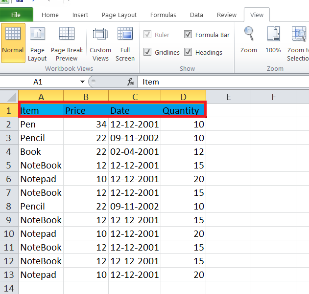
Step 1: Open your Excel worksheet.
Step 2: Select the row below the one you want to freeze.

For example, if you want to freeze the top row (row 1), you need to select row 2.
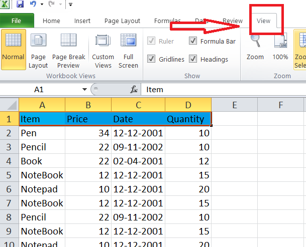
Step3: Go to the “View” tab on the Ribbon.

Step 4: Select “Freeze Top Row” if you want to freeze the top row only. Select “Freeze panes” if you want to freeze multiple rows.

ALSO READ: How to merge cells in excel
Follow these instructions to freeze rows in Excel on Mac:
Step 1: Open your Excel worksheet.
Step 2: Select the row that you want to freeze.
Similar to Windows, if you want to freeze the top row, you need to select row 2.
Step3: Go to the “View” tab on the Ribbon.
Step4: Click “Freeze Panes”.
Step 5: Select “Freeze Top Row” or “Freeze Panes,” depending on your requirement.
Watch the video here:
Quick Tips:
- Use the “Freeze Panes” option after selecting the cell below the row and to the right of the desired column if you want to freeze the top row as well as the first column.
- If you want to “Unfreeze panes,” Go to the “View” tab, click “Freeze Panes,” and then choose “Unfreeze Panes.”
💡 Ready to test your Excel knowledge?


