

When working with data in Excel, you may realize that text or numbers may not always fit inside the usual cell size. Instead of manually altering column widths and row heights, Excel’s AutoFit tool will automatically resize cells to match their content properly.
💡 Ready to test your Excel knowledge?
Method 1: Using AutoFit for a Single Column
If you wish to automatically adjust the width of one column:
Step 1: Click the column letter at the top (e.g., A).
Step 2: Navigate to the Home tab and locate the “Cells” group.
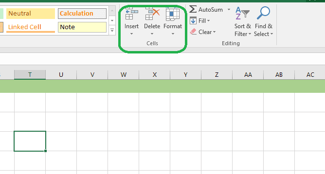
Step 3: Select Format > Autofit Column Width.
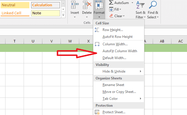
Step 4: The column will automatically resize to fit the longest piece of data.
Alternatively, double-click the column header’s right border to automatically modify it.
RELATED: How to Delete Blank Cells in Excel
Method 2: AutoFit Multiple Columns
To adjust many columns at once:
Step 1: Select all of the columns by clicking and dragging their heads.
Step 2: Double-click the right edge of any column you want to pick.
Step 3: All selected columns will be automatically resized to fit their content.
Method 3: AutoFit Row Height
If the text in a cell wraps to numerous lines or contains different font sizes, you may need to change the row height:
Step 1 : To select the row, click on the row number on the left.
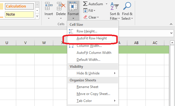
Step 2: Go to the Home tab and select Format in the “Cells” group.
Step 3: Select AutoFit Row Height, and Excel will automatically modify the row’s height.
Alternatively, double-click the row number’s bottom border to alter it instantaneously.
ALSO READ: How to Change HORIZONTAL Data to VERTICAL in Excel
Method 4: AutoFit Using Keyboard Shortcuts
For an easier method, use the following shortcut keys:
AutoFit Column Width: Alt+H+O+I
AutoFit Row Height: Alt+H+O+A
Final Thoughts
Excel’s auto-adjusting cell width and height feature ensures that your data is clearly visible and well-organized without the need for manual scaling. Whether you use the AutoFit function, double-clicking, or keyboard shortcuts, these techniques will save you time and increase spreadsheet readability.
💡 Ready to test your Excel knowledge?