How to Split Cells in Excel

You might need to use a space, a character, or something else to separate a value in a cell into two or more columns. With just a few clicks, this is easy to do. Some users, though, need to divide cells into rows. You can’t do this right out of the box in Excel, but you can use a few functions to make it work.

Learn all the different ways you can split cells in Excel by reading our step-by-step guide.

What Are Split Cells in Excel?

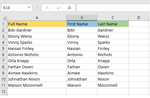
It’s useful and powerful to be able to split cells in Excel. You can split the contents of one cell across two or more cells instead of just one with this feature.

You can divide cells horizontally, making new cells to the right of the original cell, or vertically, making new cells below it. With split cells, you won’t have words cut off in the middle of a sentence. Instead, the split cells will be arranged in a grid with several cells next to each other.

When you split cells in Excel, your spreadsheet will look better because the information will be more organized and easier to read. You can also use split cells to keep long strings of words from spilling over into other columns and making them hard to read.

ALSO READ: How to Copy a Formula in Excel

How To Split Cells in Excel Using the Text to Columns Wizard

When you use the Text to Column Wizard in Excel to split cells, you can easily separate the data inside them into multiple columns. This feature figures out how to divide the data and helps you be sure you’re organising your Excel worksheet correctly.

This feature is very useful and can help you achieve your goals much faster if you need to sort, organise, or study data from outside sources.

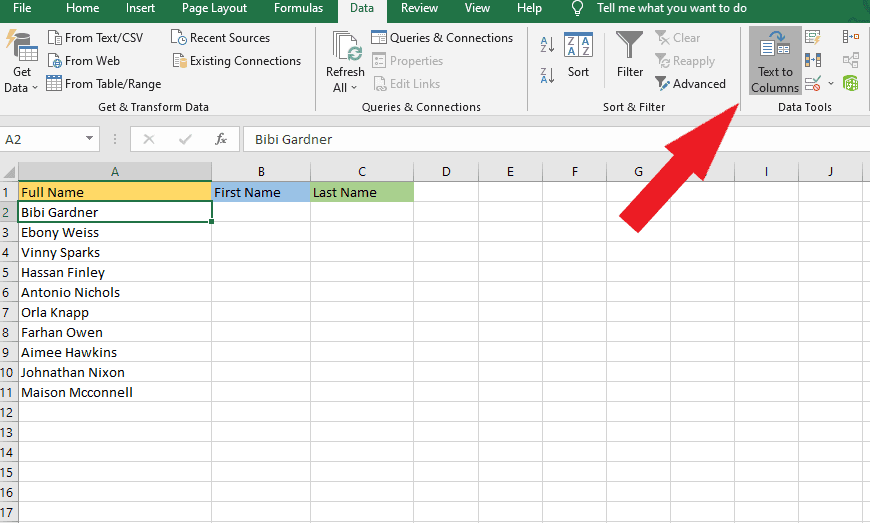
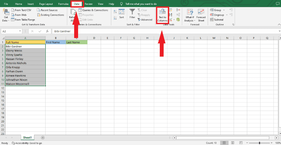
Step 1: Chose a column where you want to split the cells.

Step 2. Find the Text to Columns in the Data tab.

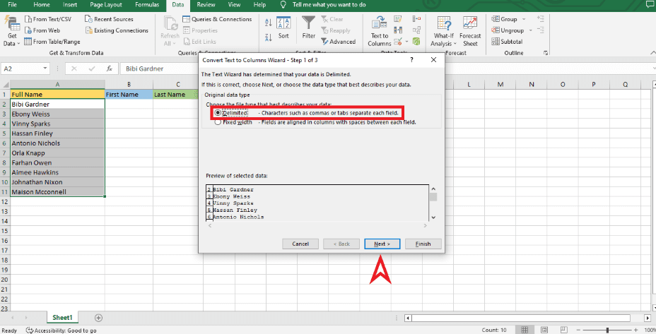
Step 3: The Convert Text to Columns Wizard opens. Choose the Delimited option that works best for your data.

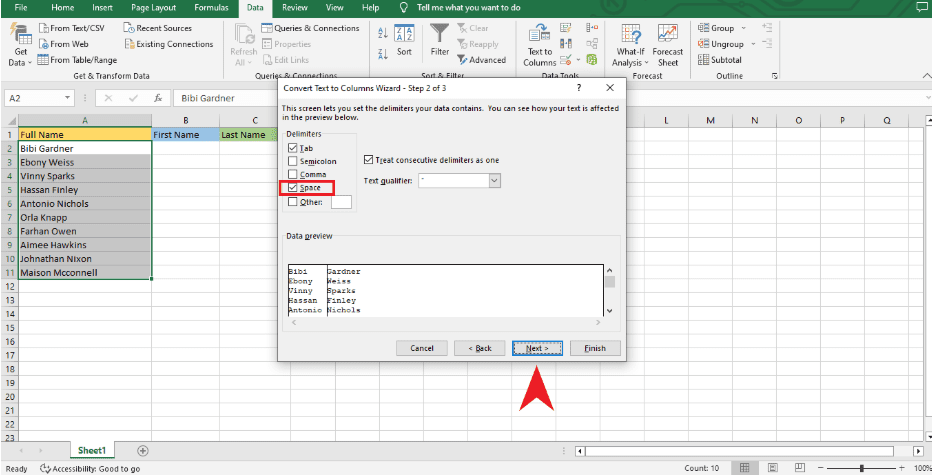
Step 4: In Step 2 of 3 of the Convert Text to Columns Wizard, pick “Space” as your Delimiter.

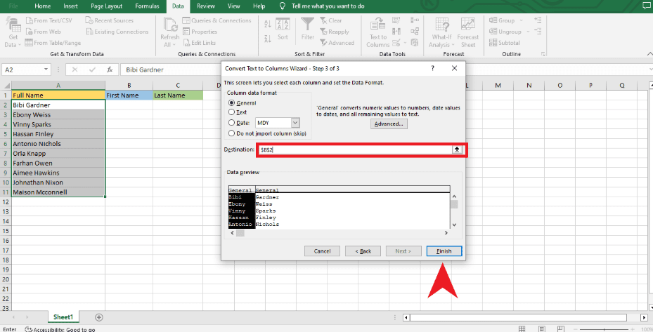
Step 5: In Convert Text to Columns Wizard Step 3 of 3, type the cell where you want the text to go.

For example, “=$B$2,” always remember to leave enough space when your data has more than one delimiter.

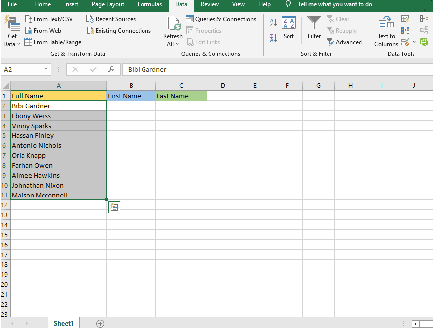
When you click “Finish,” the Text to Columns Wizard in Excel will split the cells you chose into more than one cell.

Please note that changing the names will not change the result column.

ALSO READ: How to Convert Excel to PDF

How to Split Cells in Excel Using Flash Fill

Flash Fill is a powerful tool for Excel users that lets you split cells. This tool makes it easy to split long text entries into columns when you need to.

It automatically looks for patterns in the data you put in and uses those to quickly split the data in each cell into several columns. You won’t have to split up every piece of information by hand if you split cells in Excel. This will save you time.

Flash Fill also makes sure that no data is lost and that all important information stays the same. Excel users should use this tool whenever they can because it is so useful.

Example 1:

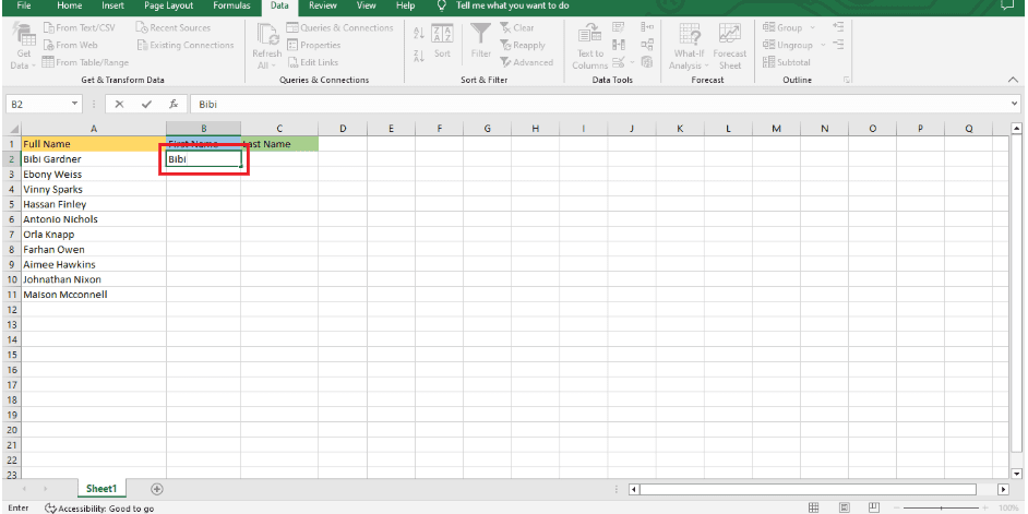
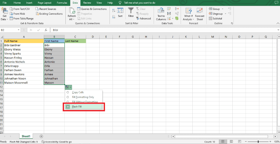
Step 1. To use the Flash fill option, type the first name in the second column.

Step 2: Move the fill handle down to the last row of the data range.

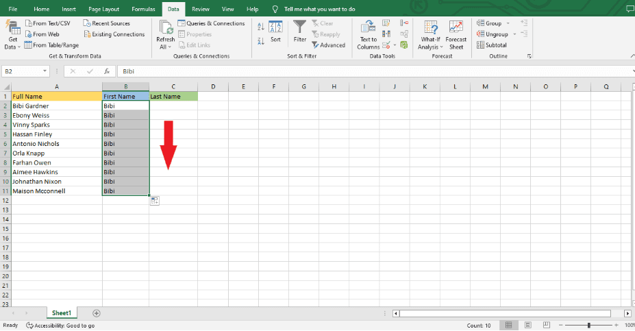
Step 3: Select the Auto Fill Options.

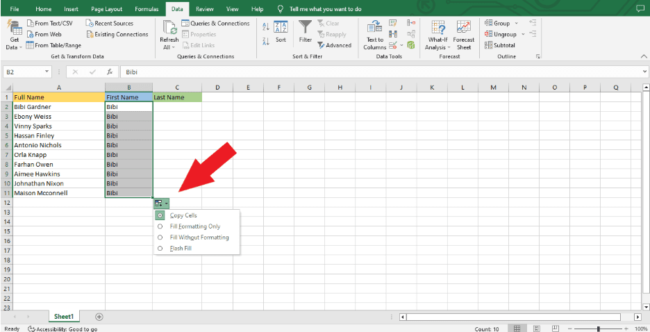
Step 4: Choose Flash Fill, and you’ll see that it fills in the first names in column b with the first names in column a.

When you want to fill in the third column using the Flash Fill Option, you need to do the same things.

Example 2:

Below is another simple way to use the Flash Fill Option.

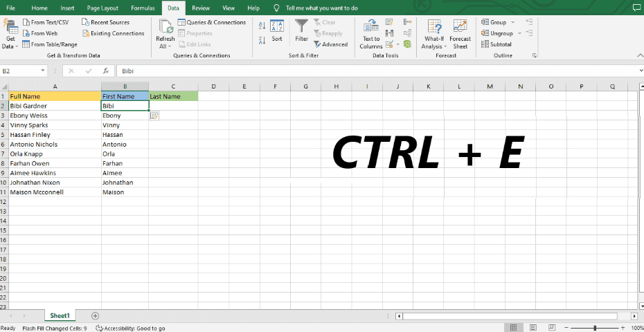
Step 1: Enter the first name.

Step 2: To Flash Fill the column, press CTRL + E.

How to split cells in Excel using Text Functions

Using text functions in Excel to split a cell is a useful search tool that can help you quickly find the information you need in a text string. You can quickly and easily search and sort through text strings with Excel functions like left, right, and mid.

You can use the left function to choose just the name part of a text string that has a person’s full name and address. This will make the name part stand out in its own cell. When you have a lot of data to work with, split cells can help you search through it. Using Excel’s text functions makes it even easier to get the data you need.

Example:

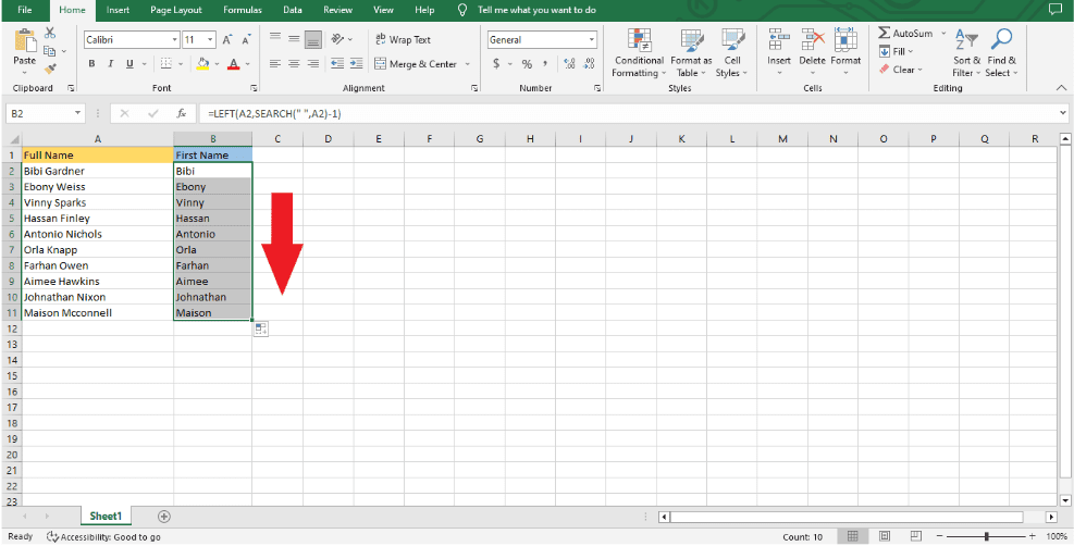
Step 1: Decide what kind of split you want to add to the data. I chose an example where the first and last names are separated by one space to make it easier to show.

Step 2: Use the SEARCH and LEFT functions to make a combination that gets the first name from a certain source.

Type the formula: =LEFT(A2,SEARCH(” “,A2)-1)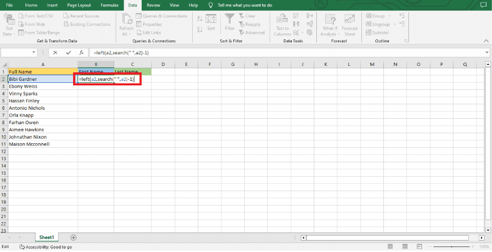

Step 3: Click on the cell where you want to type your formula, then drag the cursor down to the last range of your data.

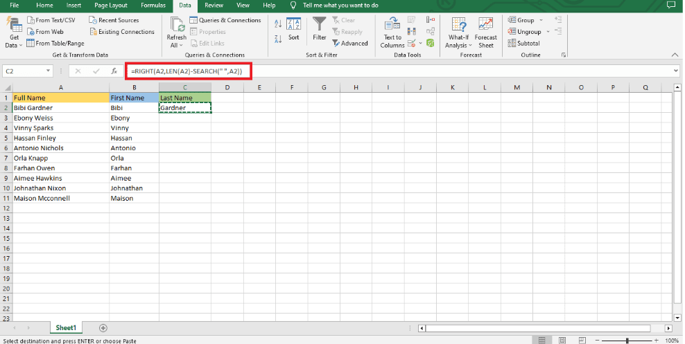
You need to do the same thing again to get the last names. But you can get data from the end of each string with the RIGHT function.

Step 1. Type the formula =RIGHT(A2,LEN(A2)-SEARCH(” “,A2)) in cell C2. 

Step 2: Click on the cell, copy the area where you type your formula, and then drag the cursor down to the end of your data.

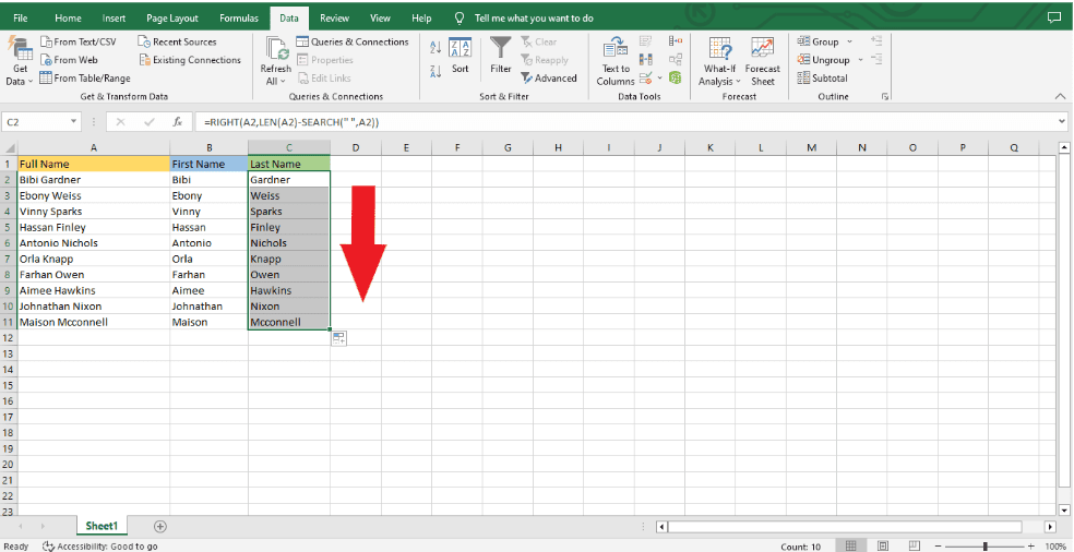
You have successfully separated the first and last names.

It is important to point out that the split is dynamic, which means that your results change automatically when you change the source data.

How To Split Cells in Excel Using Power Query

Example:

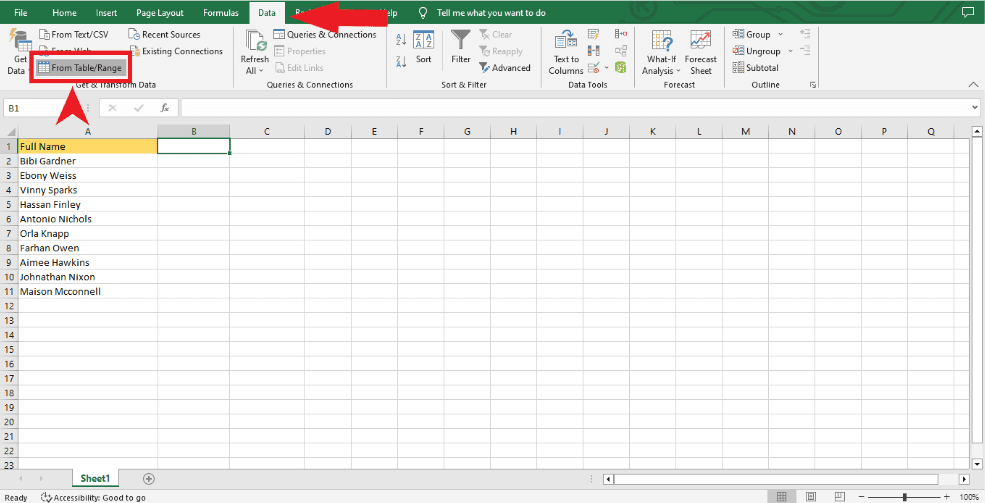
Step 1: First, choose a cell in your data set. Then, in newer versions of Excel, go to the ribbon and click on Data (tab) > From Table/Range or Data(tab)>From Sheet.

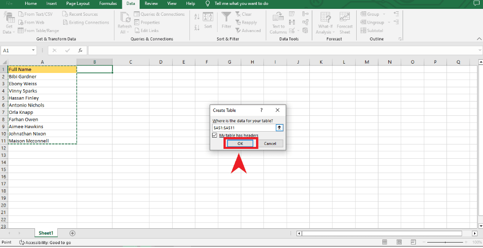
Step 2: If the cell you chose is not part of an Excel table, a Create Table window will open. Make sure that all of the rows and columns are selected and that the “My table has headers” box is checked before you click OK.

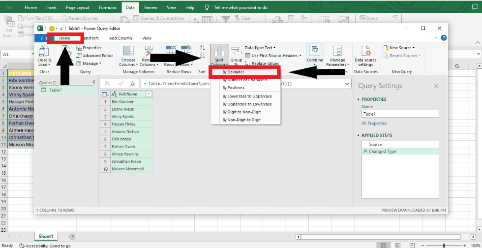
Step 3: Open the Power Query editor to see all of your data. Then, on the ribbon, go to Home > Split Column (drop-down) and choose By Delimiter to start.

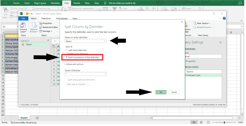
Step 4: Depending on how long your text is, different methods divide the contents of the cell into different positions. For our example, both a space and each time the separating character appears are good choices. To finish, click OK.

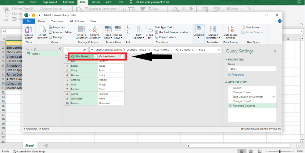
Step 5: You can now see that the names are split into two columns in the data preview window. To make them easier to find, double-click on the header and change it to “First Name” and “Last Name.”

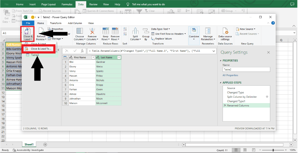
Step 6: Now you need to send the data back to Excel. To achieve this, go to Home > Close & Load (the drop-down menu) and then choose “Close & Load To…”.

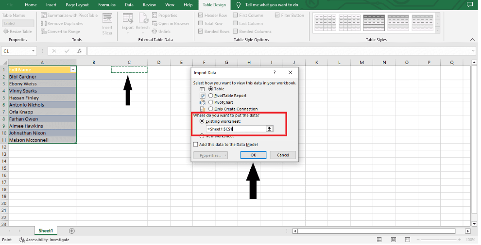
Step 7: In the Import Data dialogue box, click Table and then pick where you want to load the data. I have chosen an existing sheet at cell C1 in the example. Hit OK.

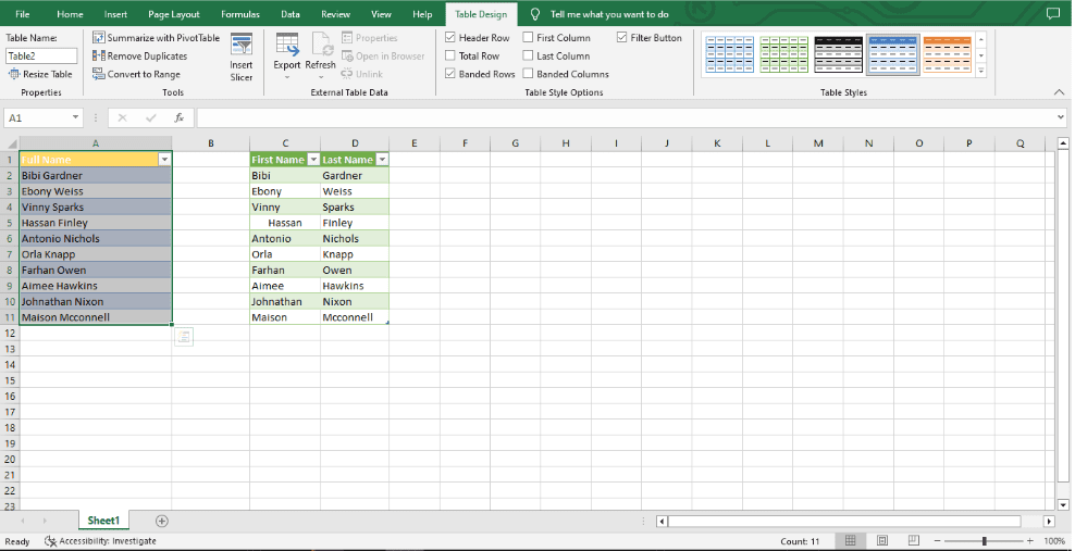
The new Power Query data will be put in the Excel cells so you can see it easily.

Conclusion

There you have it: four ways to split cells in Excel. You can see that each method has its own pros and cons, so pick the one that fits your needs the best.