
🚀 Don't Miss This Important Resource!
Explore Our Advance Xcel Tools Free !Microsoft Excel is one of the most powerful tools for dealing with data, and lookup functions play a major role in finding and retrieving information fast. For many years, users depended on functions like HLOOKUP, VLOOKUP, and INDEX + MATCH. While these functions are useful, they come with limitations that can confuse beginners and slow down expert users.
💡 Ready to test your Excel knowledge?
If you have Excel 365, Excel 2021, or newer versions, you can use XLOOKUP instead of VLOOKUP and HLOOKUP. The XLOOKUP function is much easier to use and has some extra features.
In this post, you’ll understand what XLOOKUP is, how XLOOKUP works, why it is better than earlier functions, and how to use XLOOKUP with practical examples.
What Is XLOOKUP in Excel?
XLOOKUP is an MS Excel function used to search for a value in a range or array and return a desired value from another range. It works both vertically and horizontally, making it an alternative for VLOOKUP and HLOOKUP.
Why Microsoft Introduced XLOOKUP
Older lookup functions had several problems:
- VLOOKUP could only search from left to right
- Column numbers had to be hard-coded
- Errors appeared if columns were inserted or deleted
- Exact match required extra arguments
- INDEX + MATCH was powerful but complex for beginners
XLOOKUP fixes all these issues in one simple function.
ALSO READ: VBA Excel: A Beginner’s Guide to Automating Tasks and Saving Time
How Does XLOOKUP Work Compared to VLOOKUP and INDEX/MATCH?
At its basic level, XLOOKUP performs the same task as older lookup formulas: find one value and return another. The difference resides in how much control and clarity you obtain.
With XLOOKUP, you clearly define:
- The value you are looking for
- The range to search within
- The range to return results from
This avoids the need to define column numbers or worry about whether your lookup column is on the left or right. XLOOKUP additionally defaults to exact matching, which avoids lookup mistakes that were typical with VLOOKUP’s approximate match behavior.
For users coming from INDEX/MATCH, XLOOKUP provides similar flexibility but with fewer details and a simpler structure.
Syntax of the XLOOKUP Function
The basic syntax for XLOOKUP is:
XLOOKUP(lookup_value, lookup_array, return_array, [if_not_found], [match_mode], [search_mode])Let us analyze each argument:
- Lookup_value: The value you’re looking for (such as an employee ID or product name).
- Lookup_Array: Excel will search for the lookup value in the specified range.
- Return_Array: The range that includes the value you wish to return.
- If not found (optional): If no match is found, return this value (rather than #N/A).
- Match_mode (optional): Specifies how Excel matches values. 0 – Exact match (Default)
- Search Mode (Optional): Define the search direction
XLOOKUP Basic Formula with Example
Here is the basic formula for XLOOKUP:
=XLOOKUP(A2, A:A, B:B)Example:
Imagine you have the data of employees
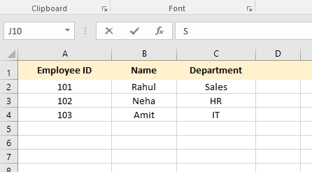
If you have to find the Department of Employee 102, use this formula:
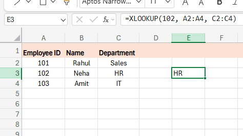
=XLOOKUP(102, A2:A4, C2:C4)
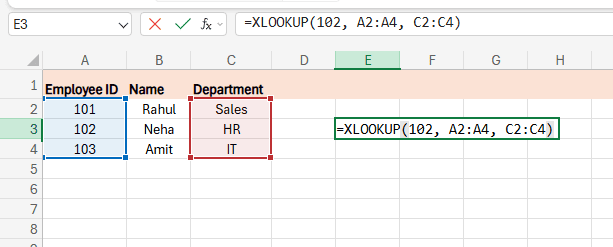
Excel looks for 102 in column A and returns its matching value from column C, which is HR.
How Does XLOOKUP Handle Missing Values and Errors?
Handling missing data is important in professional spreadsheets. XLOOKUP offers built-in error handling with the optional if_not_found argument.
Instead of covering your formula in IFERROR, you can define a fallback result right inside XLOOKUP.
XLOOKUP Error Handling Example
=XLOOKUP(A2, A:A, B:B, "Not found")If the search value does not exist, Function returns the text “Not found” instead of an error.
This enhances readability and makes formulas easier to check, especially in shared worksheets.
What Match Types Can You Use with XLOOKUP?
XLOOKUP offers several matching behaviors through the match_mode option. This allows you to execute exact matches, approximate matches, or wildcard searches.
The most usual option is exact match, which is the default. This is safer than earlier lookup functions and reduces unexpected results.
XLOOKUP Match Mode Examples:
1. Exact match (default):
=XLOOKUP(A2, A:A, B:B)2. Wildcard match:
=XLOOKUP("*"&A2&"*", A:A, B:B, , 2)3. Approximate match (next smaller value):
=XLOOKUP(A2, A:A, B:B, , -1)These features make XLOOKUP helpful for everything from text searches to graded score tables.
What Are Common Mistakes When Using XLOOKUP?
Despite its ease of use, users still make a few common mistakes when learning XLOOKUP.
One issue is mismatched ranges. The lookup array and return array must have the same size, else Excel will return an error. Another typical problem is overusing entire columns in very large datasets, which can harm performance.
It’s also essential to know that XLOOKUP is not available in older versions of Excel. If you are sharing files with users on older versions, compatibility becomes a worry.
How to use XLOOKUP with two Excel sheets?
XLOOKUP can only look up one data collection at a time.
So, we must apply nested XLOOKUP with 2 Excel sheets.
First, insert the XLOOKUP for 1 Excel sheet. As the 4th parameter, add a new XLOOKUP with the lookup and return arrays from the 2nd sheet.
Close parentheses. Press “Enter.” Then the XLOOKUP will start the search on the 1st sheet and then move to the 2nd sheet.
What Are the Limitations of XLOOKUP in Excel?
While strong, XLOOKUP has limitations. It is only available in newer Excel versions, such as Excel for Microsoft 365 and Excel 2021 and later. Workbooks with XLOOKUP will not work properly with Excel 2016 or earlier.
Additionally, XLOOKUP does not replace all use cases for lookup tables containing multiple criteria. In some cases, combining XLOOKUP with support columns or utilizing different ways may be essential.
Understanding these limitations helps you pick the correct tool for each case.
Final Thouht
XLOOKUP is one of the most essential Excel features added in recent years. It combines the top features of VLOOKUP, HLOOKUP, and INDEX + MATCH into a single, easy-to-use function. Whether you are a newbie or an expert Excel user, understanding XLOOKUP can significantly enhance your productivity and confidence while dealing with data.
💡 Ready to test your Excel knowledge?