Learn how to use the Excel XLOOKUP function with two sheets in this step-by-step tutorial. Whether you’re pulling fees from a course list, reconciling invoices, or matching equipment records, XLOOKUP makes cross-sheet lookups fast, clean, and easy to maintain.
By the end of this guide, you’ll know how to write XLOOKUP formulas that span multiple sheets — including advanced multi-criteria scenarios where you need to match on more than one column.
🔎 What you’ll learn: Basic XLOOKUP across two sheets, XLOOKUP with multiple criteria (boolean method), cross-workbook lookups, and the best alternatives for different scenarios.
Why Use XLOOKUP Across Two Sheets?
Real-world Excel data is rarely all in one place. When your data lives across two sheets (or two files), XLOOKUP is the cleanest way to bring it together without copy-pasting or manually referencing cells.
Here are the most common scenarios where this comes up:
- Student fees: Student list in Sheet 1, course price list in Sheet 2 — you want the fee for each student’s course.
- Invoice reconciliation: Invoice list in Sheet 1, payment records in Sheet 2 — you want to know which invoices are paid.
- Equipment inspections: Equipment list in Sheet 1, inspection log in Sheet 2 — you want the last inspection date for each item.
- Product pricing: Order list in Sheet 1, price catalog in Sheet 2 — you want the current price for each product ordered.
What You Need Before You Start
- Two sheets of data in the same Excel workbook — or two separate Excel files (both must be open).
- A common column between the two sheets — this is the ‘key’ XLOOKUP will use to match rows.
- Excel 2021, Microsoft 365, or Excel for the Web — XLOOKUP is not available in Excel 2019 or earlier.
⚠️ Version Note: XLOOKUP was introduced in Excel 2021 and Microsoft 365. If you’re on an older version, use VLOOKUP or INDEX+MATCH instead. See the alternatives section at the end of this guide.
ALSO READ: XLOOKUP vs VLOOKUP: Differences Between VLOOKUP and XLOOKUP in Excel
Our Example Scenario: Students & Course Fees
Throughout this tutorial, we’ll use a Students & Courses dataset. Sheet 1 contains a list of students and the course each is enrolled in. Sheet 2 contains the course fee for each course. We want to bring the fee data from Sheet 2 into Sheet 1 automatically.
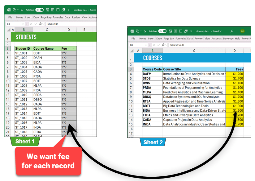
Sheet 1 (Students) and Sheet 2 (Courses) side by side — fee data needs to flow from Sheet 2 into Sheet 1
Sheet 1: Student list with Course Name column (C) and empty Fee column (D) — our target for the XLOOKUP result
XLOOKUP with Two Sheets — Basic Single-Column Lookup
Step 1: Identify the Common Column Between Both Sheets
Before writing any formula, identify which column appears in both sheets. This ‘key’ column is what XLOOKUP will use to find the matching row in Sheet 2.
In our example, the Course Name/Course Code is the common column — it appears in both the Students sheet and the Courses sheet.
💡 Quick Tip: The common column doesn’t need the same header name in both sheets — it just needs to contain the same values so XLOOKUP can make a match.
Step 2: Write the XLOOKUP Formula
Go to the sheet where you want the data to appear (Sheet 1 — Students). Click the first empty cell in the Fee column and type your XLOOKUP formula using this pattern:
=XLOOKUP(

  all cells in Sheet 1 you want to look up,

  common column in Sheet 2,

  column you want to return from Sheet 2,

  [optional: value to show if no match found]

)
For our Students & Courses example, the formula looks like this:
=XLOOKUP(C4:C43,

         Courses!B4:B15,

         Courses!D4:D15

         )
Where C4:C43 is the Course Name column in Sheet 1, Courses!B4:B15 is the Course Code column in Sheet 2, and Courses!D4:D15 is the Fee column in Sheet 2.
✅ Dynamic Spill Magic: XLOOKUP automatically fills the fee for ALL rows — you only write the formula once! No dragging, no locking references with $. This is Excel’s dynamic array / spill behavior in action.
Want to understand how Excel’s spill functionality works? Read our detailed guide on dynamic arrays and the SPILL feature in Excel for a full breakdown.
Using Excel Tables? Use Structured References Instead
If your data is in an Excel Table, use structured references — no need to select column ranges manually. Excel fills the formula down automatically:
=XLOOKUP([@Course Name], courses[name], courses[fee])
📋 Why Tables? Excel Tables auto-expand when you add new rows, so your XLOOKUP stays accurate without any maintenance. It’s the recommended approach for growing datasets.
XLOOKUP with Two Sheets and Multiple Criteria
What happens when one column isn’t enough to find the right match? For example, if the same course has different fees for in-state vs. out-of-state students, you need to match on two columns simultaneously.
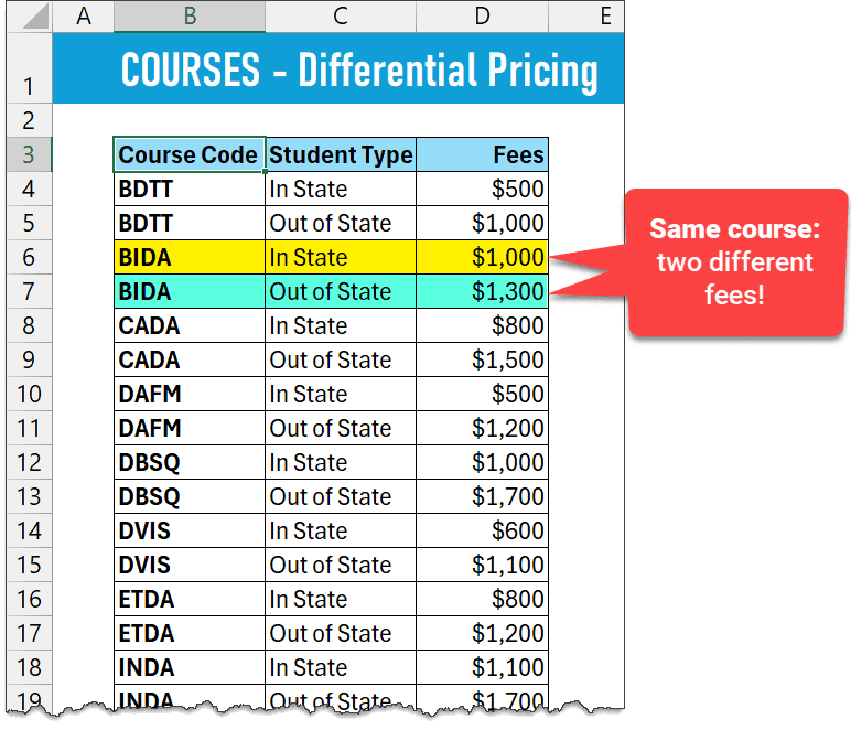
Sheet 2 (Courses — Differential Pricing): same course code (BIDA) has two different fees based on Student Type
In this scenario, your student data will also have both a Course Code column and a Student Type column — and XLOOKUP needs to check both to find the correct fee for each student.
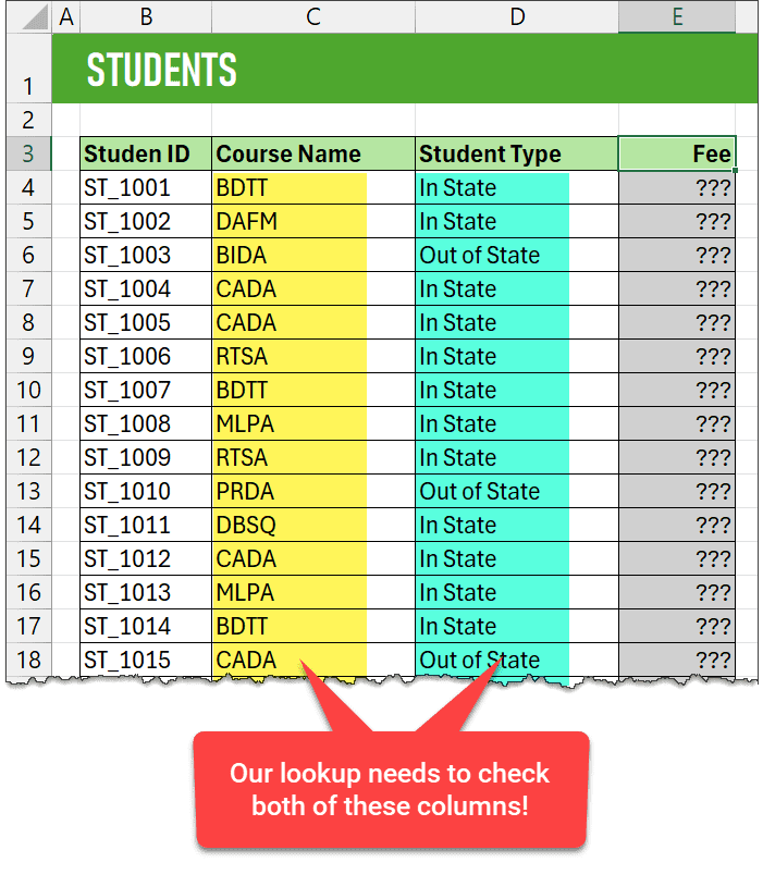
Sheet 1 (Students): Course Name (column C, yellow) and Student Type (column D, green) both need to be matched — single-column XLOOKUP won’t work here
Step 1: Identify All Common Columns
In our multi-criteria scenario, there are two common columns between the sheets:
- Course Code — Column C in Sheet 1 (Students), Column B in Sheet 2 (Courses NEW)
- Student Type — Column D in Sheet 1 (Students), Column C in Sheet 2 (Courses NEW)
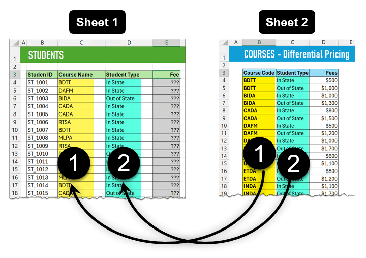
Both sheets side by side — columns 1 and 2 in each sheet must both match for XLOOKUP to return the correct fee
Step 2: Write the Multi-Criteria XLOOKUP Formula
Instead of looking up a column value directly, we use a boolean multiplication technique. The formula starts with 1 as the lookup value and builds an array of 0s and 1s by multiplying two match checks together:
=XLOOKUP(1,

  ('Courses NEW'!$B$4:$B$27=Students!C4) *

  ('Courses NEW'!$C$4:$C$27=Students!D4),

  'Courses NEW'!$D$4:$D$27)
How This Formula Works — Explained
| Part | What It Does |
| =XLOOKUP(1, …) | We look for the value 1. The formula will find a row where the match check returns 1 (true). |
| Part 1: (Sheet2!B = Sheet1!C) | Checks which rows in Sheet 2’s Course Code column match the current student’s Course Code. Returns TRUE/FALSE per row. |
| Part 2: (Sheet2!C = Sheet1!D) | Does the same check for Student Type — matches the current student’s type against Sheet 2’s Student Type column. |
| Part 1 × Part 2 | Multiplying two TRUE/FALSE arrays gives an array of 1s and 0s. Only the row where BOTH conditions match returns 1. |
| Return array | XLOOKUP finds the 1 in the result array and returns the fee from the same row in Sheet 2. |
For a deeper explanation of boolean array logic in Excel, see our guide on multiple criteria lookups in Excel at XcelNote.com.
Generic Multi-Criteria XLOOKUP Pattern
Use this template for any number of common columns. Just add more multiplication parts:
=XLOOKUP(

    1,

    (COLUMN 1 in Sheet 2 = value 1 in Sheet 1) *

    (COLUMN 2 in Sheet 2 = value 2 in Sheet 1) *

    (COLUMN 3 in Sheet 2 = value 3 in Sheet 1),

    COLUMN YOU WANT FROM SHEET 2,

    [OPTIONAL value if no match found]

)
⚠️ Important: Lock your Sheet 2 references with $ signs (e.g., $B$4:$B$27) when using the multi-criteria formula, so they don’t shift when the formula fills down to other rows.
XLOOKUP Across Two Separate Excel Files (Workbooks)
The process is exactly the same as using two sheets within one workbook — with one important rule: both files must be open at the same time for the formula to work.
- Open both Excel files before writing or refreshing the formula.
- Navigate to the other file when selecting your lookup array and return array — Excel automatically adds the file path to the formula.
- If you close the second file, the formula still shows the last calculated result, but will throw an error if you recalculate (F9) or edit the formula without the file open.
💡 Pro Tip: If you regularly pull data from another file, use Power Query instead. It works even when the source file is closed and gives you a reliable, refreshable connection.
Alternatives to XLOOKUP for Combining Data Across Sheets
XLOOKUP is the best modern option, but it’s not the only one. Here’s when to use each alternative:
| Method | Best For | Learn More |
| VLOOKUP / INDEX+MATCH | Older Excel versions that don’t support XLOOKUP. Works well for single-column lookups. | xcelnote.com/vlookup-tutorial/ |
| Power Query | Merging data from two separate files, SharePoint lists, or databases. Works when source files are closed. | xcelnote.com/power-query/ |
| Power Pivot / Data Model | Joining large tables via a common column without combining data — use pivot tables across multiple sources. | xcelnote.com/power-pivot/ |
| XLOOKUP (recommended) | Quick, modern lookups when both data sources are open. Best for single-file or small workbook scenarios. | You’re already here! 🎉 |
For a comprehensive comparison of all Excel lookup methods, check out XcelNote’s complete guide to Excel lookup functions.
XLOOKUP vs. VLOOKUP — Which Should You Use?
If you have Excel 2021 or Microsoft 365, always use XLOOKUP. Here’s why it beats VLOOKUP for cross-sheet lookups:
- No column number needed: VLOOKUP requires you to count which column number to return. XLOOKUP just references the column directly.
- Works left-to-right or right-to-left: VLOOKUP can only look right. XLOOKUP can return a column to the left of the lookup column.
- Built-in missing value handling: XLOOKUP has a 4th argument for what to show if no match is found — no need to wrap in IFERROR.
- Automatic spill: XLOOKUP can return results for an entire column at once — no drag-and-fill needed.
Frequently Asked Questions
Can XLOOKUP look up values across two different Excel files?
Yes — the process is identical to using two sheets in one workbook. The key difference is that both workbooks must be open at the same time. If you close the source file, the formula stops updating and will error on recalculation.
What is the common column in XLOOKUP?
The common column (also called a ‘key’ or ‘lookup value’) is the column that appears in both sheets with the same data — like a course code, product ID, or invoice number. XLOOKUP uses this column to find the matching row in the second sheet.
Why does my XLOOKUP return the wrong fee when I have duplicate course codes?
This happens when the same course code appears multiple times in Sheet 2 with different fees (e.g., different prices by student type). Use the multi-criteria XLOOKUP method described in this guide — match on both the course code AND the student type to get the correct result.
Do I need to lock cell references with $ when using XLOOKUP across sheets?
For the basic single-criteria XLOOKUP using a range (e.g., C4:C43), you don’t need $ signs — Excel’s dynamic spill handles it. However, for the multi-criteria boolean method, you DO need to lock the Sheet 2 references (e.g., $B$4:$B$27) so they don’t shift when filling down.
What is the XLOOKUP function syntax?
=XLOOKUP(lookup_value, lookup_array, return_array, [if_not_found], [match_mode], [search_mode])
The first three arguments are required. The remaining three are optional and cover missing-value handling, exact vs. approximate matching, and search direction.
Final Thoughts
XLOOKUP is hands-down the best way to pull data across two sheets in Excel. It’s cleaner than VLOOKUP, more flexible than INDEX+MATCH, and the multi-criteria boolean technique makes it handle even complex matching scenarios with ease.
Start with the basic single-column formula, then level up to multi-criteria matching once you’re comfortable. And if you’re working with separate files regularly, consider switching to Power Query for a more robust, file-independent solution.
Have a question about your specific XLOOKUP setup? Drop a comment below — we read every one!
For more Excel formula guides, visit XcelNote.com — your go-to resource for practical Excel tips and tutorials.