


When working with data in Excel, you may need to transpose a horizontal row to a vertical column (or vice versa). Excel has some simple methods for doing this efficiently. Here are two efficient methods for switching data from horizontal to vertical.
💡 Ready to test your Excel knowledge?
Method 1: Using Transpose (Paste Special)
The simplest way to change data orientation is to use Excel’s Transpose tool.
Step 1: Select the horizontal data range you want to convert.


Step 2: Press Ctrl + C to copy the data.
Step 3: Click on an empty cell where you want the vertical data to begin.
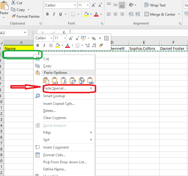
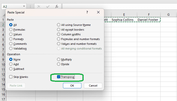
Step 4: Right-click and select Paste Special > Transpose (or press Ctrl + Alt + V, then select Transpose and click OK).


Step 5: The data will now be pasted vertically.


Method 2: Using the TRANSPOSE Function
If you want to keep the data dynamically connected (so that changes are automatically updated), use the TRANSPOSE function.
STEP 1: Select a vertical range that matches the number of horizontal cells you want to transpose.

STEP 2: Type the formula:
=TRANSPOSE(B1:F1)(Replace B1:F1 with your actual range.)


STEP 3: Press Ctrl + Shift + Enter (for older Excel versions) or simply press Enter (for newer versions with dynamic arrays).
Your data will now appear vertically and update automatically if the original data changes.

Final Thoughts
Switching data from horizontal to vertical in Excel is simple if you use the appropriate technique. The Transpose (Paste Special) approach is ideal for static data, but the TRANSPOSE function performs better when data is dynamic. For huge datasets, Power Query provides an advanced solution. Select the strategy that best meets your needs and enhance your Excel workflow!
💡 Ready to test your Excel knowledge?