

Strikethrough is one of those Excel formatting tricks that looks simple but is surprisingly hard to find. Unlike Word or Outlook, Excel doesn’t put the strikethrough button on the main ribbon—so many users don’t even know it exists.
Whether you’re marking completed tasks on a to-do list, crossing out outdated prices, or indicating canceled items in a dataset, strikethrough makes your intent visually clear at a glance.

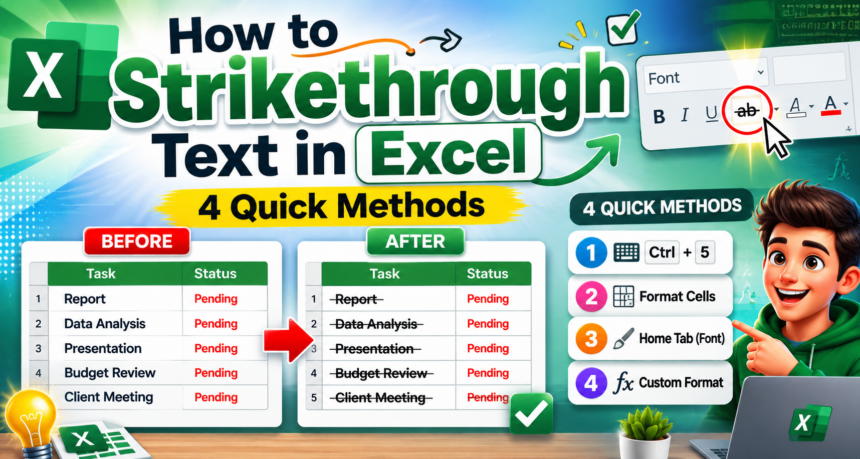
In this guide, you’ll learn 4 methods to apply strikethrough in Excel—including the fastest keyboard shortcut, the Format Cells dialog, adding it to the Quick Access Toolbar, and applying it automatically with conditional formatting.
ALSO READ: How to Make All Cells the Same Size in Excel
4 Methods at a Glance

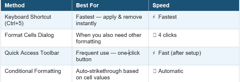
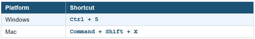
Method 1: Keyboard Shortcut — Ctrl+5 (Fastest)
The quickest way to apply strikethrough in Excel is with a dedicated keyboard shortcut. This works for both individual cells and multi-cell selections.

How to Apply Strikethrough with Ctrl+5
- Open your Excel spreadsheet.
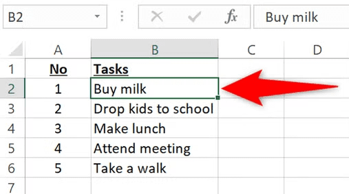
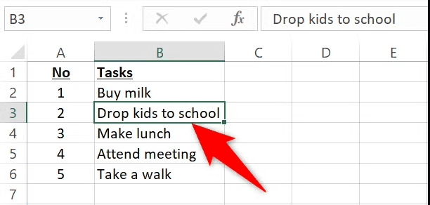
- Click the cell you want to apply strikethrough to. To select multiple cells, hold Ctrl and click each one, or drag to select a range.

3. Press Ctrl+5 on Windows or Command+Shift+X on Mac.

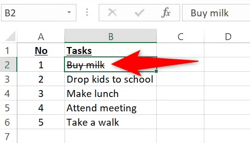
4. To remove strikethrough, select the cell again and press the same shortcut a second time. It toggles on and off. Pressing Ctrl+5 again removes the strikethrough, returning text to normal
✅ Pro Tip: You can apply strikethrough to only part of a cell’s text. Double-click the cell to enter edit mode, highlight the specific word or characters you want crossed out, then press Ctrl+5.
Method 2: Format Cells Dialog
The Format Cells dialog is the built-in graphical route to strikethrough. Strikethrough is not on the main ribbon, so this is the standard non-shortcut method. It’s also useful when you want to apply strikethrough alongside other formatting changes at the same time.
- Select the cell or range you want to format.

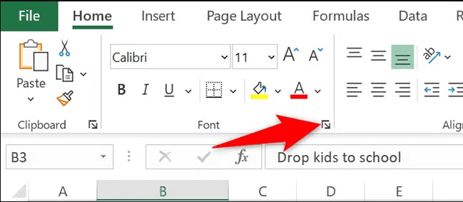
2. Go to the Home tab on the ribbon. In the Font section, click the small arrow icon in the bottom-right corner of the Font group to open the Format Cells dialog.

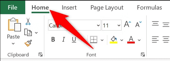
Home tab ribbon showing the small diagonal arrow in the bottom-right of the Font group

Alternatively, press Ctrl+1 to open the Format Cells dialog directly — this is the fastest route if you prefer not to use the ribbon.
- In the Format Cells dialog, click the Font tab if it isn’t already selected.
- In the Effects section, check the Strikethrough checkbox.

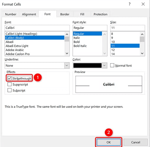
Format Cells dialog → Font tab → Effects section showing the Strikethrough checkbox
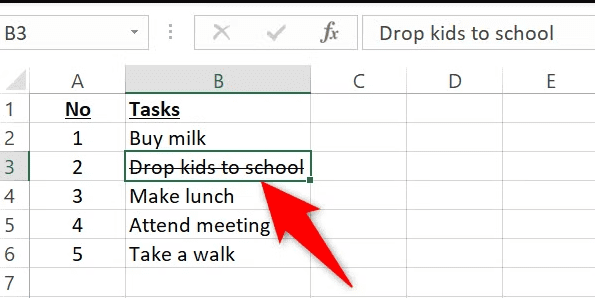
- Click OK. Strikethrough is applied to your selected cells.

💡 Bonus: The Format Cells dialog also lets you combine strikethrough with other effects like double strikethrough, superscript, or subscript—all in one step.
Method 3: Add Strikethrough to the Quick Access Toolbar
If you use strikethrough frequently, adding it as a button to the Quick Access Toolbar (QAT) means you’ll be able to apply it with a single click—no shortcuts to remember.
Setting Up the Quick Access Toolbar Button
- Click the small dropdown arrow at the end of the Quick Access Toolbar (top-left of the Excel window).
Small dropdown arrow at the right end of the Quick Access Toolbar
- Click More Commands.
QAT dropdown menu with ‘More Commands’ highlighted
- In the Excel Options dialog, change the ‘Choose commands from’ dropdown to All Commands.
Excel Options → Quick Access Toolbar → ‘Choose commands from’ set to ‘All Commands’
- Scroll down the list and find Strikethrough. Click it to select it, then click Add.
Strikethrough highlighted in All Commands list with the Add button
- Click OK. A strikethrough button (S with a line) now appears in your Quick Access Toolbar.
Quick Access Toolbar now shows the strikethrough button (S̶) for one-click access
Using the Toolbar Button
Select any cell or range, then click the strikethrough button in the Quick Access Toolbar. Click it again to remove the formatting. It works exactly like the keyboard shortcut — just with a button instead.
💡 Keyboard shortcut for QAT buttons: Once added to the QAT, you can also trigger the strikethrough button with Alt+[number] — Excel assigns a number to each QAT button automatically. Press Alt to see the numbers appear.
Method 4: Conditional Formatting (Auto-Strikethrough)
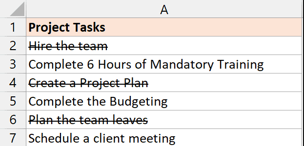
The most powerful strikethrough technique in Excel is applying it automatically using conditional formatting. For example, when you mark a task as ‘Done’ in column B, Excel can automatically cross out the task name in column A — no manual formatting needed.
Example: marking a task as Done in column B automatically strikethroughs the task name in column A
Step-by-Step: Auto-Strikethrough When a Cell Says ‘Done’
- Select the cells you want the strikethrough to appear on (e.g., the task names in column A).
Column A selected—this is where strikethrough will appear automatically
- Go to Home → Conditional Formatting → New Rule.
Conditional Formatting dropdown with ‘New Rule’ highlighted
- In the New Formatting Rule dialog, select ‘Use a formula to determine which cells to format.’
New Formatting Rule dialog—’Use a formula to determine which cells to format’ selected
- Enter your formula. For example, if your status column is B, enter:
=B1=”Done”
Formula =B1=”Done” entered in the conditional formatting formula box
- Click the Format button to open the Format Cells dialog.
- On the Font tab, check the Strikethrough checkbox and click OK.
Format Cells dialog within conditional formatting — Strikethrough checkbox enabled
- Click OK to close the New Formatting Rule dialog and apply the rule.
Tasks marked as ‘Done’ in column B now automatically show strikethrough in column A
✅ Why this is powerful: Conditional formatting strikethrough updates automatically as your data changes. Mark a task as done, and the strikethrough appears instantly—mark it as in progress, and it disappears just as fast.
To learn more about conditional formatting rules in Excel, visit XcelNote.com’s Conditional Formatting Guide for a full walkthrough.
Useful Tips for Strikethrough in Excel
- Apply to part of a cell: Double-click to enter edit mode, select specific characters, then press Ctrl+5. Only those characters will be crossed out.
- Strikethrough multiple cells at once: Select a range (or hold Ctrl to select non-adjacent cells), then apply the shortcut or dialog. All selected cells update together.
- Strikethrough doesn’t affect formulas: Applying strikethrough to a cell with a formula only changes the visual display—the formula still calculates normally.
- Combine with cell color: Pair strikethrough with a gray fill color using conditional formatting to make completed items look truly ‘done.’
- Works in charts too: If a cell with strikethrough feeds into a chart, the chart data is unaffected — only the cell display changes.
Frequently Asked Questions
What is the strikethrough shortcut in Excel?
On Windows, the keyboard shortcut is Ctrl+5. On Mac, it’s Command+Shift+X. Press the shortcut once to apply and again to remove.
Why can’t I find the strikethrough button in the Excel ribbon?
Unlike Word, Excel doesn’t include a strikethrough button on the default Home tab ribbon. It’s available in the Format Cells dialog (Ctrl+1 → Font → Strikethrough) or can be added to the Quick Access Toolbar as described in Method 3.
Can I apply strikethrough to just part of the text in a cell?
Yes. Double-click the cell to enter edit mode, then highlight only the characters you want to cross out. Press Ctrl+5 and only the selected text will have strikethrough — the rest of the cell stays normal.
How do I remove strikethrough from a cell in Excel?
Select the cell and press Ctrl+5 again — the shortcut toggles the formatting on and off. Alternatively, open Format Cells (Ctrl+1), uncheck the Strikethrough checkbox, and click OK.
Can I make strikethrough apply automatically in Excel?
Yes — use conditional formatting. Create a rule that triggers strikethrough formatting when a cell meets a specific condition (e.g., when a status column says ‘Done’). See Method 4 above for full step-by-step instructions.
Final Thoughts
Strikethrough in Excel is more useful than most people realize—especially for task tracking, version control, and visual data management. The keyboard shortcut (Ctrl+5) is the fastest way to apply it, while the conditional formatting method gives you a fully automated solution that keeps your spreadsheet up to date without any extra clicks.
Add it to your Quick Access Toolbar if you use it regularly, and explore the conditional formatting route if you want your spreadsheet to do the work for you.